MMM-With-Carryover-And-Saturation
MMM-With-Carryover-And-Saturation.RmdData
Impressions Data
glimpse(mmm_imps)
#> Rows: 200
#> Columns: 5
#> $ Date       <date> 2018-01-07, 2018-01-14, 2018-01-21, 2018-01-28, 2018-02-04…
#> $ mi_tv      <dbl> 344275.4, 0.0, 0.0, 0.0, 0.0, 204905.0, 0.0, 243839.5, 0.0,…
#> $ mi_radio   <dbl> 0.00, 17206.08, 21155.95, 13623.15, 0.00, 19578.15, 0.00, 1…
#> $ mi_banners <dbl> 0.000, 3731.596, 2217.981, 0.000, 4274.270, 2801.566, 3329.…
#> $ kpi_sales  <dbl> 9779.80, 13245.19, 12022.66, 8846.95, 9797.07, 13527.65, 96…
Spend Data
glimpse(mmm_spend)
#> Rows: 200
#> Columns: 5
#> $ Date       <date> 2018-01-07, 2018-01-14, 2018-01-21, 2018-01-28, 2018-02-04…
#> $ mi_tv      <dbl> 13528.10, 0.00, 0.00, 0.00, 0.00, 8045.44, 0.00, 9697.29, 0…
#> $ mi_radio   <dbl> 0.00, 5349.65, 4235.86, 3562.21, 0.00, 4310.55, 0.00, 4478.…
#> $ mi_banners <dbl> 0.00, 2218.93, 2046.96, 0.00, 2187.29, 1992.98, 2253.02, 20…
#> $ kpi_sales  <dbl> 9779.80, 13245.19, 12022.66, 8846.95, 9797.07, 13527.65, 96…
Model Recipes
Recipe without transformation
ln_init_mmm <-
  recipe(kpi_sales ~ ., data = mmm_imps) |>
  add_role(c(mi_tv, mi_radio, mi_banners), new_role = "mi") |>
  update_role(Date, new_role = "temp") |>
  update_role_requirements("temp", bake = FALSE)
Recipe with transformations with default hyperparameters
cs_init_mmm <-
  recipe(kpi_sales ~ ., data = mmm_imps) |>
  add_role(c(mi_tv, mi_radio, mi_banners), new_role = "mi") |>
  update_role(Date, new_role = "temp") |>
  update_role_requirements("temp", bake = FALSE) |>
  step_geometric_adstock(mi_banners) |>
  step_geometric_adstock(mi_tv) |>
  step_geometric_adstock(mi_radio) |>
  step_hill_saturation(mi_banners, max_ref = TRUE) |>
  step_hill_saturation(mi_tv, max_ref = TRUE) |>
  step_hill_saturation(mi_radio, max_ref = TRUE)
dl_init_mmm <-
  recipe(kpi_sales ~ ., data = mmm_imps) |>
  add_role(c(mi_tv, mi_radio, mi_banners), new_role = "mi") |>
  update_role(Date, new_role = "temp") |>
  update_role_requirements("temp", bake = FALSE) |>
  step_delayed_adstock(mi_banners) |>
  step_delayed_adstock(mi_tv) |>
  step_delayed_adstock(mi_radio) |>
  step_hill_saturation(mi_banners, max_ref = TRUE) |>
  step_hill_saturation(mi_tv, max_ref = TRUE) |>
  step_hill_saturation(mi_radio, max_ref = TRUE)
wb_init_mmm <-
  recipe(kpi_sales ~ ., data = mmm_imps) |>
  add_role(c(mi_tv, mi_radio, mi_banners), new_role = "mi") |>
  update_role(Date, new_role = "temp") |>
  update_role_requirements("temp", bake = FALSE) |>
  step_weibull_adstock(mi_banners) |>
  step_delayed_adstock(mi_tv) |>
  step_delayed_adstock(mi_radio) |>
  step_hill_saturation(mi_banners, max_ref = TRUE) |>
  step_hill_saturation(mi_tv, max_ref = TRUE) |>
  step_hill_saturation(mi_radio, max_ref = TRUE)
Recipe with tuned carryover and saturation transformations
cs_tuned_mmm <-
  recipe(kpi_sales ~ ., data = mmm_imps) |>
  add_role(c(mi_tv, mi_radio, mi_banners), new_role = "mi") |>
  update_role(Date, new_role = "temp") |>
  update_role_requirements("temp", bake = FALSE) |>
  step_geometric_adstock(mi_banners, decay = 0.432, max_carryover = 1) |>
  step_hill_saturation(mi_banners, shape = 1.30, max_ref = TRUE) |>
  step_geometric_adstock(mi_tv, decay = 0.0181, max_carryover = 8) |>
  step_hill_saturation(mi_tv, shape = 0.783, max_ref = TRUE) |>
  step_geometric_adstock(mi_radio, decay = 0.193, max_carryover = 1) |>
  step_hill_saturation(mi_radio, shape = 1.06, max_ref = TRUE)
Setup Workflows
Using the same linear regression with the Bayesian estimation engine.
lm_mod <- linear_reg() |> set_engine("stan")

ln_init_wflow <-
  workflow() |>
  add_model(lm_mod) |>
  add_recipe(ln_init_mmm)

cs_init_wflow <-
  workflow() |>
  add_model(lm_mod) |>
  add_recipe(cs_init_mmm)

dl_init_wflow <-
  workflow() |>
  add_model(lm_mod) |>
  add_recipe(dl_init_mmm)

wb_init_wflow <-
  workflow() |>
  add_model(lm_mod) |>
  add_recipe(wb_init_mmm)

cs_tuned_wflow <-
  workflow() |>
  add_model(lm_mod) |>
  add_recipe(cs_tuned_mmm)
Fitting Models / Running Workflows
ln_init_fit <- ln_init_wflow |> fit(data = mmm_imps)
cs_init_fit <- cs_init_wflow |> fit(data = mmm_imps)
dl_init_fit <- dl_init_wflow |> fit(data = mmm_imps)
wb_init_fit <- wb_init_wflow |> fit(data = mmm_imps)
cs_tuned_fit <- cs_tuned_wflow |> fit(data = mmm_imps)
Use tidy to extract fitted parameters
tidy(ln_init_fit, conf.int = TRUE)
#> # A tibble: 4 × 5
#>   term         estimate  std.error  conf.low conf.high
#>   <chr>           <dbl>      <dbl>     <dbl>     <dbl>
#> 1 (Intercept) 6992.     220.       6651.     7359.
#> 2 mi_tv          0.0138   0.000796    0.0125    0.0152
#> 3 mi_radio       0.131    0.0107      0.114     0.148
#> 4 mi_banners     0.661    0.0672      0.553     0.767
tidy(cs_init_fit, conf.int = TRUE)
#> # A tibble: 4 × 5
#>   term         estimate std.error  conf.low conf.high
#>   <chr>           <dbl>     <dbl>     <dbl>     <dbl>
#> 1 (Intercept) 1760.     402.      1114.     2425.
#> 2 mi_tv          0.0281   0.00119    0.0261    0.0300
#> 3 mi_radio       0.252    0.0218     0.217     0.288
#> 4 mi_banners     1.92     0.165      1.65      2.20
tidy(dl_init_fit, conf.int = TRUE)
#> # A tibble: 4 × 5
#>   term         estimate std.error  conf.low conf.high
#>   <chr>           <dbl>     <dbl>     <dbl>     <dbl>
#> 1 (Intercept) 5376.     594.      4382.     6366.
#> 2 mi_tv          0.0202   0.00153    0.0176    0.0227
#> 3 mi_radio       0.145    0.0336     0.0902    0.200
#> 4 mi_banners     0.941    0.239      0.518     1.32
tidy(wb_init_fit, conf.int = TRUE)
#> # A tibble: 4 × 5
#>   term         estimate std.error  conf.low conf.high
#>   <chr>           <dbl>     <dbl>     <dbl>     <dbl>
#> 1 (Intercept) 4107.     502.      3288.     4917.
#> 2 mi_tv          0.0204   0.00144    0.0181    0.0227
#> 3 mi_radio       0.154    0.0295     0.106     0.201
#> 4 mi_banners     1.50     0.190      1.19      1.81
tidy(cs_tuned_fit, conf.int = TRUE)
#> # A tibble: 4 × 5
#>   term         estimate  std.error  conf.low conf.high
#>   <chr>           <dbl>      <dbl>     <dbl>     <dbl>
#> 1 (Intercept) 6563.     197.       6238.     6883.
#> 2 mi_tv          0.0162   0.000718    0.0150    0.0174
#> 3 mi_radio       0.116    0.00791     0.103     0.129
#> 4 mi_banners     0.854    0.0736      0.733     0.972
Post-Modeling
Named List of trained models
models <- list(
  ln_init_fit = ln_init_fit,
  cs_init_fit = cs_init_fit,
  dl_init_fit = dl_init_fit,
  wb_init_fit = wb_init_fit,
  cs_tuned_fit = cs_tuned_fit
  )
Model Decomposition
model_decomps <- decompose(models, new_data = mmm_imps, spend_data = mmm_spend)
model_decomps
#> # A tibble: 5 × 5
#>   model        workflow   decomp             roi              pred
#>   <chr>        <list>     <list>             <list>           <list>
#> 1 ln_init_fit  <workflow> <tibble [800 × 9]> <tibble [4 × 4]> <tibble [200 × 1]>
#> 2 cs_init_fit  <workflow> <tibble [800 × 9]> <tibble [4 × 4]> <tibble [200 × 1]>
#> 3 dl_init_fit  <workflow> <tibble [800 × 9]> <tibble [4 × 4]> <tibble [200 × 1]>
#> 4 wb_init_fit  <workflow> <tibble [800 × 9]> <tibble [4 × 4]> <tibble [200 × 1]>
#> 5 cs_tuned_fit <workflow> <tibble [800 × 9]> <tibble [4 × 4]> <tibble [200 × 1]>
Model Metrics & Fit
model_metrics(model_decomps, new_data = mmm_imps)
#> # A tibble: 5 × 4
#>   model        workflow     rsq  mape
#>   <chr>        <list>     <dbl> <dbl>
#> 1 cs_tuned_fit <workflow> 0.819  9.42
#> 2 cs_init_fit  <workflow> 0.814  9.90
#> 3 ln_init_fit  <workflow> 0.752 11.2
#> 4 wb_init_fit  <workflow> 0.618 13.7
#> 5 dl_init_fit  <workflow> 0.533 15.4
plot_model_fit(model_decomps)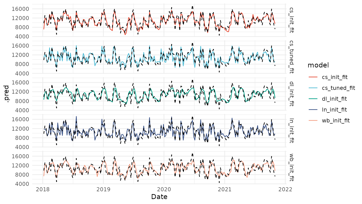
Contributions
Contribution percent breakdown
plot_base_contribution(model_decomps)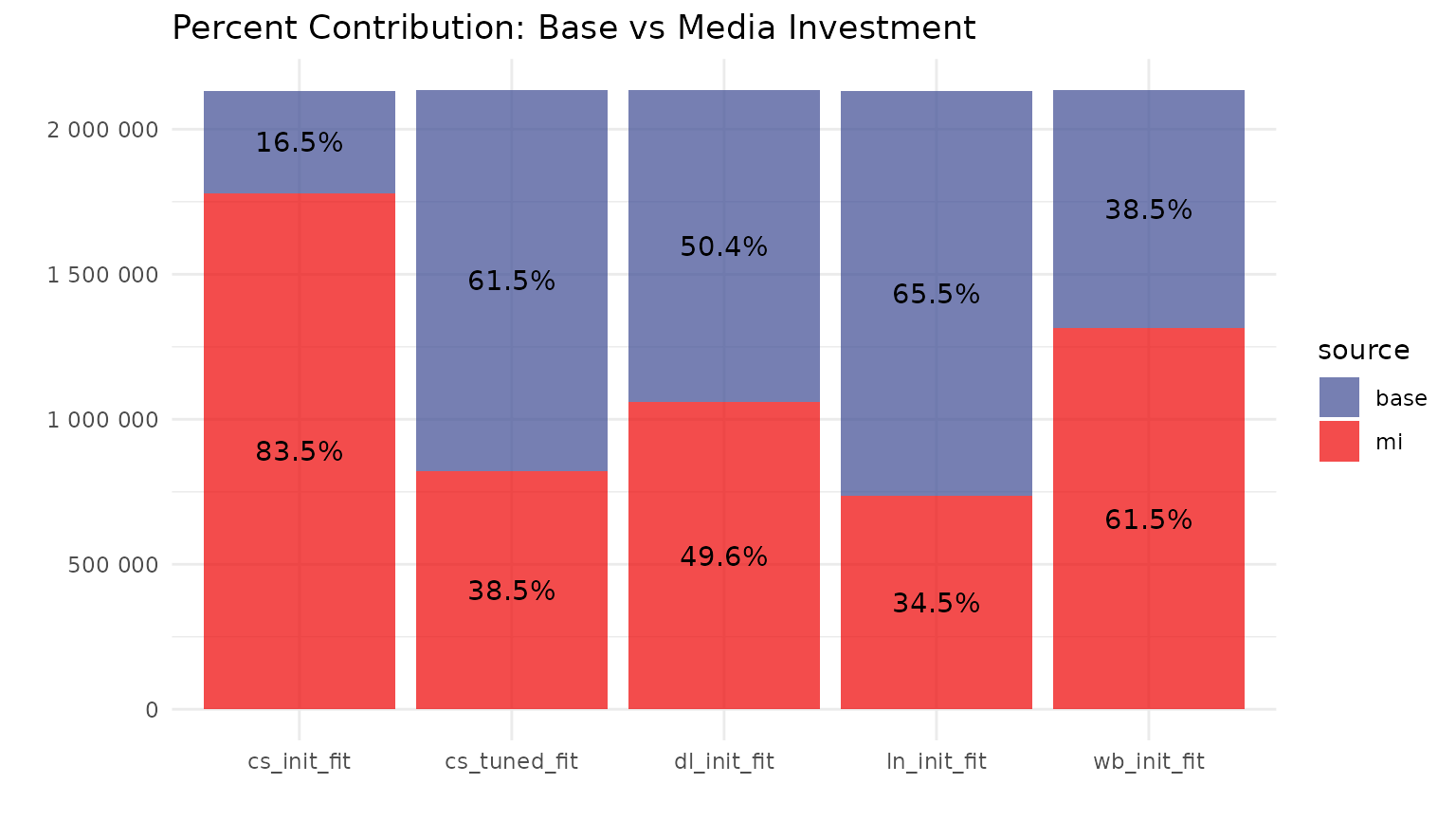
plot_channel_contribution(model_decomps)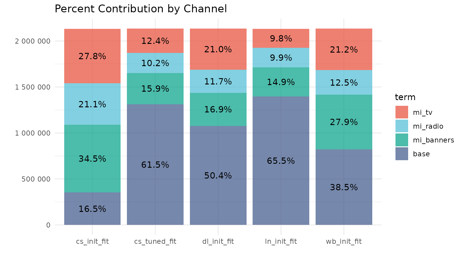
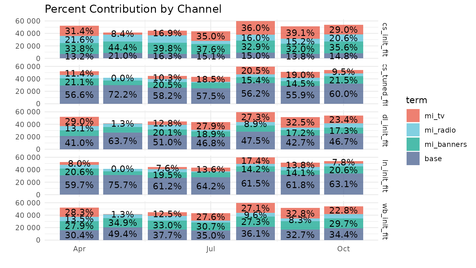
model_decomps |>
  filter(model == "cs_tuned_fit") |>
  plot_channel_contribution_month(
    begin_date = "2021-04-01",
    end_date = "2022-01-01"
    )
Channel contrbution volume and ROIs
channel_metrics(model_decomps)
#> # A tibble: 4 × 11
#>   term   sales_ln_init_fit sales_cs_init_fit sales_dl_init_fit sales_wb_init_fit
#>   <chr>              <dbl>             <dbl>             <dbl>             <dbl>
#> 1 base            1397307.           352848.          1075685.           821563.
#> 2 mi_tv            208236.           594139.           447573.           451876.
#> 3 mi_ra…           210475.           449617.           250609.           266390.
#> 4 mi_ba…           316862.           736554.           361497.           594800.
#> # ℹ 6 more variables: sales_cs_tuned_fit <dbl>, ROI_ln_init_fit <dbl>,
#> #   ROI_cs_init_fit <dbl>, ROI_dl_init_fit <dbl>, ROI_wb_init_fit <dbl>,
#> #   ROI_cs_tuned_fit <dbl>
Plot ROIs
plot_roi(model_decomps)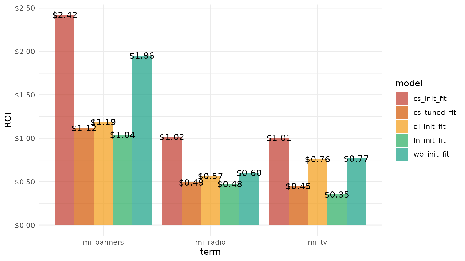
Response Curves
Generate response from model decomposition
response <- response_curves(model_decomps)
response
#> # A tibble: 24,000 × 8
#>    model       var        var_shape var_nu mid_point_x mid_point_y     x      y
#>    <chr>       <chr>          <dbl>  <dbl>       <dbl>       <dbl> <dbl>  <dbl>
#>  1 cs_init_fit mi_banners         1      1     304145.     736554.    0      0
#>  2 cs_init_fit mi_banners         1      1     304145.     736554.  304.  1472.
#>  3 cs_init_fit mi_banners         1      1     304145.     736554.  609.  2942.
#>  4 cs_init_fit mi_banners         1      1     304145.     736554.  913.  4408.
#>  5 cs_init_fit mi_banners         1      1     304145.     736554. 1217.  5872.
#>  6 cs_init_fit mi_banners         1      1     304145.     736554. 1521.  7333.
#>  7 cs_init_fit mi_banners         1      1     304145.     736554. 1826.  8790.
#>  8 cs_init_fit mi_banners         1      1     304145.     736554. 2130. 10245.
#>  9 cs_init_fit mi_banners         1      1     304145.     736554. 2434. 11697.
#> 10 cs_init_fit mi_banners         1      1     304145.     736554. 2739. 13146.
#> # ℹ 23,990 more rows
Visualize response curves
plot_response_curves(response)Estimate mROI and ROI from the response curves
mroi(response)
#> # A tibble: 12 × 4
#> # Groups:   var [3]
#>    var        model          ROI  mROI
#>    <chr>      <chr>        <dbl> <dbl>
#>  1 mi_banners cs_init_fit  2.42  1.21
#>  2 mi_banners cs_tuned_fit 1.12  0.727
#>  3 mi_banners dl_init_fit  1.19  0.595
#>  4 mi_banners wb_init_fit  1.96  0.978
#>  5 mi_radio   cs_init_fit  1.02  0.508
#>  6 mi_radio   cs_tuned_fit 0.493 0.261
#>  7 mi_radio   dl_init_fit  0.566 0.283
#>  8 mi_radio   wb_init_fit  0.602 0.301
#>  9 mi_tv      cs_init_fit  1.01  0.504
#> 10 mi_tv      cs_tuned_fit 0.449 0.176
#> 11 mi_tv      dl_init_fit  0.760 0.380
#> 12 mi_tv      wb_init_fit  0.767 0.384