Fitting a Response Model: A Simulated Example • mrmopt

library(mrmopt)
library(brms)
#> Loading required package: Rcpp
#> Loading 'brms' package (version 2.23.0). Useful instructions
#> can be found by typing help('brms'). A more detailed introduction
#> to the package is available through vignette('brms_overview').
#> 
#> Attaching package: 'brms'
#> The following object is masked from 'package:stats':
#> 
#>     ar
library(purrr)
library(gt)
library(dplyr)
#> 
#> Attaching package: 'dplyr'
#> The following objects are masked from 'package:stats':
#> 
#>     filter, lag
#> The following objects are masked from 'package:base':
#> 
#>     intersect, setdiff, setequal, union
library(ggplot2)
library(patchwork)


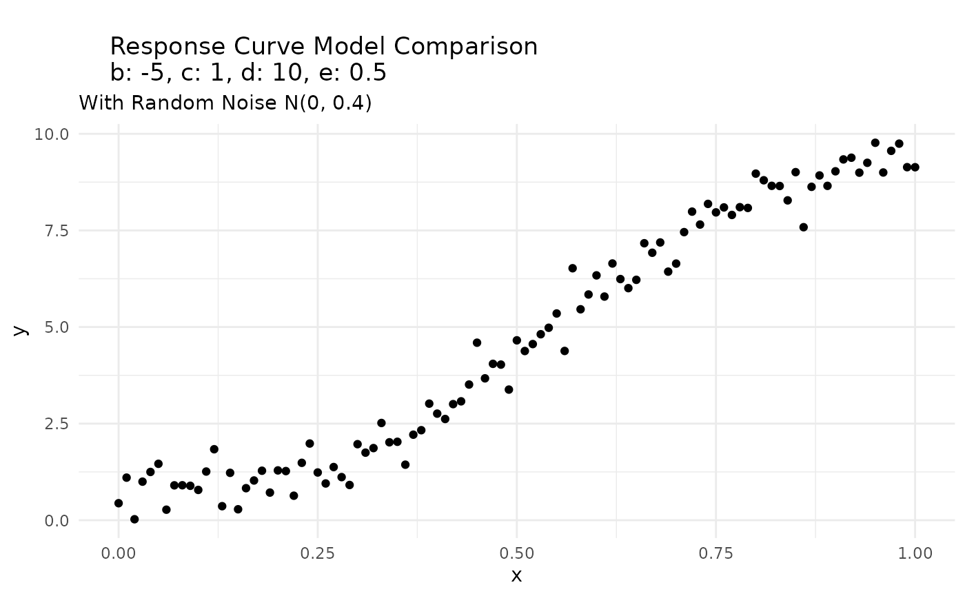
x_values <- seq(0, 1, by = 0.01)

b <- -5
c <- 1
d <- 10
e <- 0.5

y_response = rm_Gompertz(x_values, b, c, d, e) + rnorm(length(x_values), mean = 0, sd = 0.4)

response_df <- bind_cols(
  x = x_values,
  y = y_response
)



response_df |>
  ggplot(aes(x, y)) +
  geom_point() +
  labs(title = paste0("
    Response Curve Model Comparison
    ", "b: ", b, ", c: ", c, ", d: ", d, ", e: ", e),
    subtitle = "With Random Noise N(0, 0.4)" 
  ) +
  theme_minimal()

response_fit = 
  fit_response(
    data = response_df,
    x = "x",
    y = "y",
    type = "gompertz",
    auto = TRUE,
    # prior = c(
    #   prior(normal(-5, 10), nlpar = "b", lb = -10, ub = 0),
    #   prior(normal(0, 5), nlpar = "c", ub = 4.9),
    #   prior(normal(10, 5), nlpar = "d", lb = 5.1),
    #   prior(normal(0.6, 2), nlpar = "e")
    # ),
    chains = 2,
    iter = 2000, 
    warmup = 1000,
    seed = 007,
    control = list(adapt_delta = 0.90)
  )
#> y ~ c + (d - c) * exp(-exp(b * (x - e))) 
#> b ~ 1
#> c ~ 1
#> d ~ 1
#> e ~ 1
#> 
#> SAMPLING FOR MODEL 'anon_model' NOW (CHAIN 1).
#> Chain 1: 
#> Chain 1: Gradient evaluation took 0.000126 seconds
#> Chain 1: 1000 transitions using 10 leapfrog steps per transition would take 1.26 seconds.
#> Chain 1: Adjust your expectations accordingly!
#> Chain 1: 
#> Chain 1: 
#> Chain 1: Iteration:    1 / 2000 [  0%]  (Warmup)
#> Chain 1: Iteration:  200 / 2000 [ 10%]  (Warmup)
#> Chain 1: Iteration:  400 / 2000 [ 20%]  (Warmup)
#> Chain 1: Iteration:  600 / 2000 [ 30%]  (Warmup)
#> Chain 1: Iteration:  800 / 2000 [ 40%]  (Warmup)
#> Chain 1: Iteration: 1000 / 2000 [ 50%]  (Warmup)
#> Chain 1: Iteration: 1001 / 2000 [ 50%]  (Sampling)
#> Chain 1: Iteration: 1200 / 2000 [ 60%]  (Sampling)
#> Chain 1: Iteration: 1400 / 2000 [ 70%]  (Sampling)
#> Chain 1: Iteration: 1600 / 2000 [ 80%]  (Sampling)
#> Chain 1: Iteration: 1800 / 2000 [ 90%]  (Sampling)
#> Chain 1: Iteration: 2000 / 2000 [100%]  (Sampling)
#> Chain 1: 
#> Chain 1:  Elapsed Time: 1.04 seconds (Warm-up)
#> Chain 1:                1.056 seconds (Sampling)
#> Chain 1:                2.096 seconds (Total)
#> Chain 1: 
#> 
#> SAMPLING FOR MODEL 'anon_model' NOW (CHAIN 2).
#> Chain 2: 
#> Chain 2: Gradient evaluation took 7.9e-05 seconds
#> Chain 2: 1000 transitions using 10 leapfrog steps per transition would take 0.79 seconds.
#> Chain 2: Adjust your expectations accordingly!
#> Chain 2: 
#> Chain 2: 
#> Chain 2: Iteration:    1 / 2000 [  0%]  (Warmup)
#> Chain 2: Iteration:  200 / 2000 [ 10%]  (Warmup)
#> Chain 2: Iteration:  400 / 2000 [ 20%]  (Warmup)
#> Chain 2: Iteration:  600 / 2000 [ 30%]  (Warmup)
#> Chain 2: Iteration:  800 / 2000 [ 40%]  (Warmup)
#> Chain 2: Iteration: 1000 / 2000 [ 50%]  (Warmup)
#> Chain 2: Iteration: 1001 / 2000 [ 50%]  (Sampling)
#> Chain 2: Iteration: 1200 / 2000 [ 60%]  (Sampling)
#> Chain 2: Iteration: 1400 / 2000 [ 70%]  (Sampling)
#> Chain 2: Iteration: 1600 / 2000 [ 80%]  (Sampling)
#> Chain 2: Iteration: 1800 / 2000 [ 90%]  (Sampling)
#> Chain 2: Iteration: 2000 / 2000 [100%]  (Sampling)
#> Chain 2: 
#> Chain 2:  Elapsed Time: 1.284 seconds (Warm-up)
#> Chain 2:                1.024 seconds (Sampling)
#> Chain 2:                2.308 seconds (Total)
#> Chain 2:

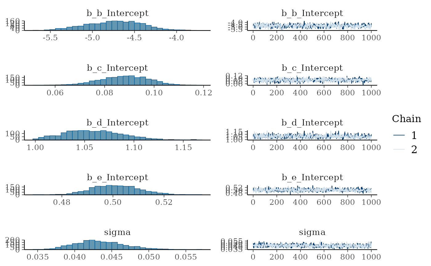
summary(response_fit)
#>  Family: gaussian 
#>   Links: mu = identity 
#> Formula: y ~ c + (d - c) * exp(-exp(b * (x - e))) 
#>          b ~ 1
#>          c ~ 1
#>          d ~ 1
#>          e ~ 1
#>    Data: data (Number of observations: 101) 
#>   Draws: 2 chains, each with iter = 2000; warmup = 1000; thin = 1;
#>          total post-warmup draws = 2000
#> 
#> Regression Coefficients:
#>             Estimate Est.Error l-95% CI u-95% CI Rhat Bulk_ESS Tail_ESS
#> b_Intercept    -4.74      0.33    -5.40    -4.12 1.01      576      794
#> c_Intercept     0.09      0.01     0.07     0.11 1.01      950     1090
#> d_Intercept     1.06      0.03     1.01     1.12 1.01      542      435
#> e_Intercept     0.50      0.01     0.48     0.52 1.00      924      943
#> 
#> Further Distributional Parameters:
#>       Estimate Est.Error l-95% CI u-95% CI Rhat Bulk_ESS Tail_ESS
#> sigma     0.04      0.00     0.04     0.05 1.00      894      842
#> 
#> Draws were sampled using sampling(NUTS). For each parameter, Bulk_ESS
#> and Tail_ESS are effective sample size measures, and Rhat is the potential
#> scale reduction factor on split chains (at convergence, Rhat = 1).

plot(response_fit)

pp_check(response_fit)

mrm_plot_response(response_fit) +
  mrm_plot_response(response_fit, scaled = FALSE) +
  mrm_plot_response(response_fit, markup = TRUE) +
  plot_layout(ncol = 2)

bind_cols(
  actual = c(b, c, d, e),
  mrm_params(response_fit) |> 
    map(~round(unlist(.x), 2)) |> 
    as_tibble()
) |> 
  gt::gt() |> 
  gt::tab_header(
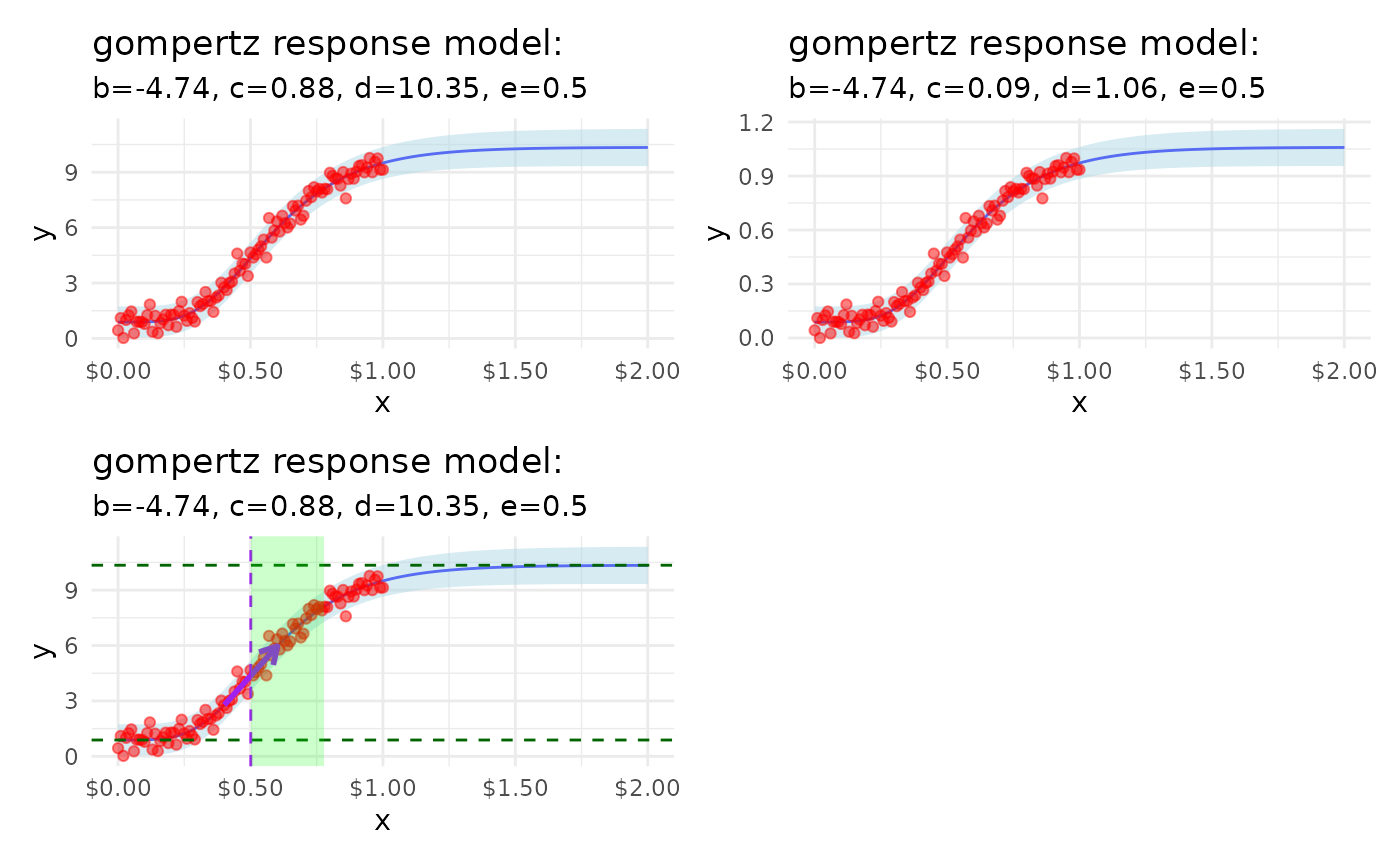
    title = "Parameter Estimates vs Actual Values",
    subtitle = "Using the Gompertz Response Model"
  )

actual	center	lower	upper
Parameter Estimates vs Actual Values
Using the Gompertz Response Model
-5.0	-4.74	-5.40	-4.12
1.0	0.88	0.68	1.06
10.0	10.35	9.85	10.95
0.5	0.50	0.48	0.52

mrm_params_table(response_fit, scaled = FALSE) |> 
  gt::tab_header(
    title = "Parameter Estimates Table",
    subtitle = "Using the Gompertz Response Model"
  )

Parameter	center	lower	upper
Parameter Estimates Table
Using the Gompertz Response Model
b (growth rate)	-4.741645	-5.398366	-4.123516
c (lower asymptote)	0.08800686	0.06760201	0.1062646
d (upper asymptote)	1.059448	1.008309	1.120964
e (inflection point)	0.5012417	0.4843928	0.5204534

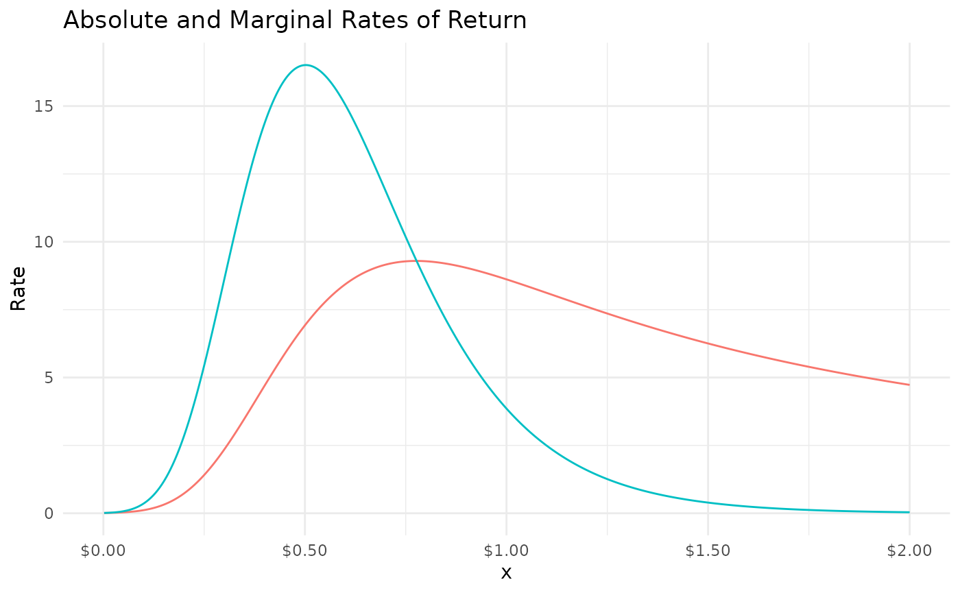
response = mrm_infer(response_fit, length.out = 100)

head(response) |> 
  gt::gt() |>
  gt::tab_header(
    title = "Inferred Response Data",
    subtitle = "Using the Gompertz Response Model"
  ) |>
  gt::fmt_number(
    columns = tidyselect::everything(),
    decimals = 2
  )

x	Estimate	Est.Error	Q2.5	Q97.5	center	lower	upper	type	resp_var	input_var	ar	mr	cp	cp_lower	ar_lower	mr_lower	ar_upper	mr_upper	cp_upper
Inferred Response Data
Using the Gompertz Response Model
0.00	0.89	0.43	0.07	1.73	0.88	0.03	1.74	gompertz	y	x	NaN	NA	NaN	NaN	NaN	NA	NaN	NA	NaN
0.02	0.89	0.43	0.00	1.77	0.88	0.03	1.74	gompertz	y	x	0.02	0.02	53.35	60.60	0.03	0.03	0.00	0.00	3,718.16
0.04	0.88	0.43	0.04	1.74	0.88	0.03	1.74	gompertz	y	x	0.03	0.04	32.26	36.65	0.04	0.06	0.01	0.02	76.30
0.06	0.90	0.43	0.01	1.74	0.89	0.03	1.74	gompertz	y	x	0.05	0.08	19.52	22.17	0.06	0.10	0.03	0.06	28.98
0.08	0.90	0.43	0.01	1.74	0.89	0.04	1.74	gompertz	y	x	0.07	0.16	11.99	13.62	0.09	0.18	0.05	0.14	14.49
0.10	0.90	0.43	0.03	1.79	0.89	0.04	1.74	gompertz	y	x	0.12	0.29	7.54	8.56	0.14	0.31	0.10	0.27	8.17

mrm_plot_return(response_fit)