This post is about my new R package ConversionPath which aims to put together a number of useful tools for analyzing conversion path data commonly encountered in digital marketing and MTA analysis.
If you want to try it out you can download the development version from my github
devtools::install_github("bdshaff/conversionpath")Estimate a Transition Matrix from Data
library(ConversionPath)
set.seed(007)
fit_transition_matrix performs the simple task of estimating a transition matrix. To demo this I will use a sample data-set digital_conversion_path that is included with the package. The estimation method is MLE, though only the actual transition probabilities are computed. (No Standard Errors).
Example Data-set
data("digital_conversion_path")
head(digital_conversion_path, 10) |> gt::gt()| path | conv_count | drop_count |
|---|---|---|
| Paid Search | 184 | 920 |
| Organic Social | 174 | 1218 |
| Programmatic | 162 | 1296 |
| Organic Search | 158 | 1106 |
| Online-Video | 142 | 1420 |
| Paid Social | 129 | 1161 |
| Paid Search > Programmatic | 55 | 385 |
| Organic Social > Paid Search | 36 | 288 |
| Organic Search > Programmatic | 33 | 297 |
| Programmatic > Paid Social | 33 | 198 |
tail(digital_conversion_path, 10) |> gt::gt()| path | conv_count | drop_count |
|---|---|---|
| Programmatic > Paid Social > Organic Search > Programmatic | 1 | 9 |
| Programmatic > Paid Social > Organic Social | 1 | 7 |
| Programmatic > Paid Social > Organic Social > Paid Social > Organic Search > Programmatic > Paid Search > Programmatic > Organic Search | 1 | 6 |
| Programmatic > Paid Social > Paid Search | 1 | 5 |
| Programmatic > Paid Social > Paid Search > Programmatic > Online-Video | 1 | 7 |
| Programmatic > Paid Social > Paid Search > Programmatic > Paid Search | 1 | 10 |
| Programmatic > Paid Social > Programmatic > Online-Video > Organic Search | 1 | 9 |
| Programmatic > Paid Social > Programmatic > Organic Search > Online-Video | 1 | 5 |
| Programmatic > Paid Social > Programmatic > Organic Search > Online-Video > Organic Search | 1 | 5 |
| Programmatic > Paid Social > Programmatic > Organic Social > Paid Social | 1 | 10 |
- Extract a list of paths from the data-set using
extract_path_list
conv_count = digital_conversion_path$conv_count
drop_count = digital_conversion_path$drop_count
P = extract_path_list(digital_conversion_path)
Here is a sample from this list
P[sample(1:length(P),5)]## [[1]]
## [1] "Organic Search" "Online-Video" "Paid Search"
##
## [[2]]
## [1] "Online-Video" "Organic Social" "Online-Video" "Programmatic"
## [5] "Paid Social" "Online-Video"
##
## [[3]]
## [1] "Organic Search" "Programmatic" "Organic Search" "Paid Social"
##
## [[4]]
## [1] "Organic Social" "Paid Social" "Paid Search"
##
## [[5]]
## [1] "Paid Search" "Paid Social" "Online-Video" "Paid Social"- Fit the transition matrix by providing the path list, vector of total conversions per path, and a vector of total non-conversions per path.
M = fit_transition_matrix(P, conv_count, drop_count)## [1] "Start: Online-Video"
## [1] "END: Online-Video"
## [1] "Start: Organic Search"
## [1] "END: Organic Search"
## [1] "Start: Organic Social"
## [1] "END: Organic Social"
## [1] "Start: Paid Search"
## [1] "END: Paid Search"
## [1] "Start: Paid Social"
## [1] "END: Paid Social"
## [1] "Start: Programmatic"
## [1] "END: Programmatic"round(M, 3)## start conv drop Online-Video Organic Search Organic Social
## start 0 0.000 0.000 0.188 0.141 0.164
## conv 0 1.000 0.000 0.000 0.000 0.000
## drop 0 0.000 1.000 0.000 0.000 0.000
## Online-Video 0 0.044 0.361 0.000 0.151 0.071
## Organic Search 0 0.047 0.352 0.119 0.000 0.048
## Organic Social 0 0.045 0.315 0.076 0.081 0.000
## Paid Search 0 0.053 0.347 0.031 0.028 0.121
## Paid Social 0 0.045 0.348 0.168 0.201 0.045
## Programmatic 0 0.052 0.393 0.111 0.120 0.063
## Paid Search Paid Social Programmatic
## start 0.189 0.154 0.164
## conv 0.000 0.000 0.000
## drop 0.000 0.000 0.000
## Online-Video 0.087 0.133 0.154
## Organic Search 0.057 0.166 0.211
## Organic Social 0.182 0.134 0.167
## Paid Search 0.000 0.190 0.230
## Paid Social 0.047 0.000 0.147
## Programmatic 0.092 0.170 0.000The result is the matrix you see above. The format of the matrix is “proper” for conversion data analysis in that the non accessible start state, and the absorbing conv and drop states are implicitly added to the transition matrix. To be proper the following conditions are enforced:
- first column is a row of probabilities for the starting point of the path.
- first column is all 0s indicating that the starting position is not accessible from any state in the markov chain.
- the second and third row/column form a 2x2 identity sub matrix designating the absorbing conversion and non-conversion states.
- the matrix is a proper transition matrix i.e. square and all rows sum to 1.
Comparison and Integration with ChannelAttribution
If you are using the ChannelAttribution::markov_model, by specifying the argument out_more = TRUE we can get back a transition matrix in a long format, and indexed touch-points. With the transition_matrix_from_markov_model function we can generate a “proper” transition matrix. This may be useful if you want to use the matrix for visualization and simulation.
library(ChannelAttribution)

mcm = markov_model(digital_conversion_path,
                   var_path = "path",
                   var_conv = "conv_count",
                   var_null = "drop_count",
                   out_more = TRUE,
                   verbose = FALSE)

MC = transition_matrix_from_markov_model(mcm)
round(MC[colnames(M),colnames(M)], 3)
## start conv drop Online-Video Organic Search Organic Social
## start 0 0.000 0.000 0.188 0.155 0.174
## conv 0 1.000 0.000 0.000 0.000 0.000
## drop 0 0.000 1.000 0.000 0.000 0.000
## Online-Video 0 0.044 0.361 0.000 0.151 0.071
## Organic Search 0 0.047 0.352 0.119 0.000 0.048
## Organic Social 0 0.045 0.315 0.076 0.081 0.000
## Paid Search 0 0.053 0.347 0.031 0.028 0.121
## Paid Social 0 0.045 0.348 0.168 0.201 0.045
## Programmatic 0 0.052 0.393 0.111 0.120 0.063
## Paid Search Paid Social Programmatic
## start 0.171 0.154 0.157
## conv 0.000 0.000 0.000
## drop 0.000 0.000 0.000
## Online-Video 0.087 0.133 0.154
## Organic Search 0.057 0.166 0.211
## Organic Social 0.182 0.134 0.167
## Paid Search 0.000 0.190 0.230
## Paid Social 0.047 0.000 0.147
## Programmatic 0.092 0.170 0.000Visualization
Transition Matrix
Simple plot of the transition matrix:
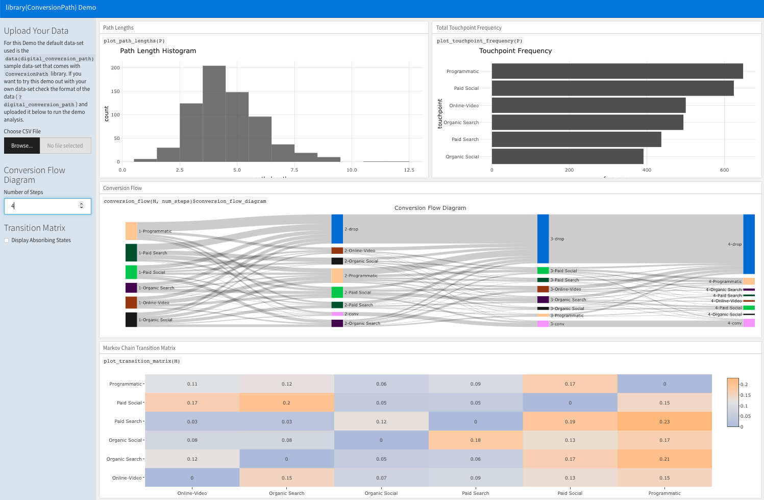
plot_transition_matrix(M)Adding the absorbing states into the picture:
plot_transition_matrix(M, full = TRUE)Conversion Flow
The conversion_flow function runs a simulation with a given number of simulated paths num_sim = 20 each with a given number of steps num_steps = 4. We have the simulated table, and the conversion flow diagram returned.
S = conversion_flow(M, num_steps = 4, num_sim = 50)
S$conversion_flow_diagram
More paths:
S = conversion_flow(M, num_steps = 4, num_sim = 300)
S$conversion_flow_diagram
More steps:
S = conversion_flow(M, num_steps = 6, num_sim = 300)
S$conversion_flow_diagram
Path Data EDA
Some other useful function for visualizing the actual path data and the derived path_list
plot_path_lengths(P)plot_touchpoint_frequency(P)More
There is certainly more functionality to come, and more functionality that is already present. Specifically, some simulation functions that are behind the conversion_flow function. The actual design of the functions will probably also change. One thing is for sure, there are more EDA plots and summaries that will be added to work with conversion path type of data.
If you have a small data-set with which this may be tested feel free to try and run by uploading data to the demo shiny app:
http://bdshaff.shinyapps.io/CP-FlexDash