CNN for Binary Grayscale Image Classification with Keras in R

Package Build 2021-06-10 21 min read

Binary Image Classification with Keras in R (Apple M1 Chip)

The exercise is done on hardware with an Apple M1 Chip and using R interface to Keras. This means that the versions of R, Python, TensorFlow and Keras are all versions that run natively on the M1 Chip. If you prefer to use R and use an M1 mac then here are a few useful links:

To then make this available in R you just need to use reticulate::use_condaenv and point to the environment where the Python and TF were setup.

library(tensorflow)
library(keras)
library(purrr)
library(imager)
library(stringr)

reticulate::use_condaenv("~/miniforge3/envs/python38/")

Data

For this exercise I am using a data-set from Kaggle which was used for the Intel Image Classification competition. The original task is a multiclass classification with building, street, forest, glacier, mountain, sea as labels. For the first model I simplified the task to a binary classification and used gray-scale images even though colored images are available.

Here is the structure of the data in this project. Building, Street are grouped to make a first class, and forest, glacier, mountain, sea are grouped to make the second class.

fs::dir_tree(paste0(path, "/data"), recurse = 2, regexp = "train|test")

## ~/Documents/Ben's Data Science/Intel Image Classifiction/data
## ├── test
## │   ├── city
## │   │   ├── buildings
## │   │   └── street
## │   └── nature
## │       ├── forest
## │       ├── glacier
## │       ├── mountain
## │       └── sea
## └── train
##     ├── city
##     │   ├── buildings
##     │   └── street
##     └── nature
##         ├── forest
##         ├── glacier
##         ├── mountain
##         └── sea

Loading Image Data in R

There are a couple of ways to read in the images into R. One way is to use imager::load.image function. The advantage is that we get an object of class cimg which is easy to manipulate, plot, and cast to an array. For ML and for building models in Keras using keras::image_load() and keras::image_to_array() is more convenient because we can specify if we want to use gray-scale images and the target size. Images all need to be of the same dimension. We expect 150x150 images in this data, but some images are in fact of a different size and would need to be further processed or excluded. keras::image_load() very conveniently helps us take care of this issue.

train_image_files = list.files(paste0(path,"/data/train"), 
                               recursive = TRUE, 
                               full.names = TRUE)

train_labels = map_chr(train_image_files, ~ifelse(
  str_detect(.x,"city"), "city/building","nature"))

y_train = to_categorical(as.numeric(as.factor(train_labels)), num_classes = 3)[,2:3]

test_image_files = list.files(paste0(path,"/data/test"), 
                              recursive = TRUE, 
                              full.names = TRUE)
test_labels = map_chr(test_image_files, ~ifelse(
  str_detect(.x,"city"), "city/building","nature"))

y_test = to_categorical(as.numeric(as.factor(test_labels)), num_classes = 3)[,2:3]

train_data = map(train_image_files, 
                ~image_load(.x, target_size = c(150,150), grayscale = TRUE) %>% 
                  image_to_array() %>% 
                  divide_by(255)
                )

test_data = map(test_image_files, 
                ~image_load(.x, target_size = c(150,150), grayscale = TRUE) %>% 
                  image_to_array() %>% 
                  divide_by(255)
                )

When the data is loaded using purrr::map we get back a list of images. This is very convenient for certain use cases but for Keras we need to use arrays which are higher dimensional matrices. Thankfully it is not very difficult to restructure the data into one big array and give it the right dimensions using base R functions array unlist and aperm.

X_test = 
  array(unlist(test_data), 
        dim = c(150, 150, 1, length(test_data))) %>% 
  aperm(c(4,1,2,3))

X_train = 
  array(unlist(train_data), 
        dim = c(150, 150, 1, length(train_data))) %>% 
  aperm(c(4,1,2,3))

Sample Images

To visualize a sample image from either the test of train sets it is easy to simply slice the resultant array of data and cast back to cimg.

par(mfrow = c(1,2), mar = c(1,1,1,1))
as.cimg(X_test[2000, , , ])  %>% 
  imrotate(90) %>% 
  plot(axes = FALSE, main = test_labels[2000])

as.cimg(X_train[1, , , ]) %>% 
  imrotate(90) %>% 
  plot(axes = FALSE, main = train_labels[1])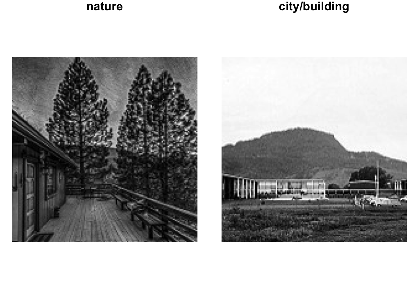

Convolutional Neural Network (CNN)

Define Model

Images are represented as 2D or 3D (if colored) arrays which can be reshaped to 1D vectors. We can train a model using this 1D vector representation but even intuitively this feel like we are giving up important information. CNNs, or networks with convolutional layers are particularly useful when it comes to images because they allow us to retain and learn the importance of spacial relationships within the samples.

model = keras_model_sequential()
model %>% 
  layer_conv_2d(120, kernel_size = 3, strides = 2, activation = "relu", 
                input_shape = c(150, 150, 1)) %>%
  layer_max_pooling_2d(2) %>%
  layer_conv_2d(60, kernel_size = 3, strides = 2, activation = "relu") %>%
  layer_conv_2d(60, kernel_size = 3, strides = 2, activation = "relu") %>%
  layer_max_pooling_2d(2) %>%
  layer_conv_2d(40, kernel_size = 3, strides = 2, activation = "relu") %>%
  layer_flatten() %>%
  #a dense layer with two nodes and sigmoid binary activation to produce probabilities
  layer_dense(2, activation = "sigmoid")

summary(model)

## Model: "sequential"
## ________________________________________________________________________________
## Layer (type)                        Output Shape                    Param #     
## ================================================================================
## conv2d_3 (Conv2D)                   (None, 74, 74, 120)             1200        
## ________________________________________________________________________________
## max_pooling2d_1 (MaxPooling2D)      (None, 37, 37, 120)             0           
## ________________________________________________________________________________
## conv2d_2 (Conv2D)                   (None, 18, 18, 60)              64860       
## ________________________________________________________________________________
## conv2d_1 (Conv2D)                   (None, 8, 8, 60)                32460       
## ________________________________________________________________________________
## max_pooling2d (MaxPooling2D)        (None, 4, 4, 60)                0           
## ________________________________________________________________________________
## conv2d (Conv2D)                     (None, 1, 1, 40)                21640       
## ________________________________________________________________________________
## flatten (Flatten)                   (None, 40)                      0           
## ________________________________________________________________________________
## dense (Dense)                       (None, 2)                       82          
## ================================================================================
## Total params: 120,242
## Trainable params: 120,242
## Non-trainable params: 0
## ________________________________________________________________________________

Compile and Fit

Defining the loss function and the optimization procedure are likewise very simple to do thanks to Keras.

model %>% 
  compile(
    loss = "binary_crossentropy",
    optimizer = "adam",
    metrics = "accuracy"
  )

Here we are using the test data for validation during the learning process.

history =
  model %>%
  fit(
    x = X_train, y = y_train,
    validation_data = list(X_test, y_test),
    epochs = 10,
    batch_size = 10
  )

Training History

From the training history we can see that the model reaches a relatively good level of accuracy and perhaps begins to over-fit somewhat by the 4th epoch. From the plot we see that the model reaches a ~94% prediction accuracy on the test set of images and a slightly higher ~95% prediction accuracy on the train set.

plotly::ggplotly(
  plot(history)
)

Save

For some reason before using the model for prediction on my machine I need to save it and load it each time. HDF5 format also seems to work more reliably with R markdown.

save_model_hdf5(model, paste0(path,"/tf_models/binary_gray_img_classification"))

Evaluation

Model Accuracy

We saw from the training history plot that the prediction accuracy was ~94%. We can recreate this and then go a little bit deeper in evaluating the model using a simple confusion matrix.

First lets get the predicted labels:

smodel = load_model_hdf5(paste0(path,"/tf_models/binary_gray_img_classification"), 
                         compile = TRUE)


tpred = vector(mode = "character", length = dim(X_test)[1])
for(i in 1:dim(X_test)[1]){
  #pick the lable with the max predicted probability
  tpred[i] =  c("city/building","nature")[
    which.max(smodel %>% predict(X_test[i, , , ,drop = FALSE]))
    ]
}


conf = table(tpred, test_labels)/length(tpred)
round(conf,2)

##                test_labels
## tpred           city/building nature
##   city/building          0.26   0.02
##   nature                 0.05   0.67

Looking at the confusion matrix above we see that 31% of the time we predict a city/building label and 69% of the time we predict a nature label. We can tell by summing the diagonal that the overall accuracy is indeed 95%, yet we also see that our model struggles more with correctly identifying a city/building image.

this is the probability of predicting nature while the true label is city/building. \[ P(Nature|City) = 0.02/0.29 = 6.9\% \] on the other hand the likelihood of making the opposite error is

\[ P(City|Nature) = 0.03/0.66 = 4.5\% \] Essentially the model likes to play it safe and predict nature more often. When we look to validate the model it will be slightly more likely to falsely classify an image of a building/city as nature

Examples of Miss-Classification

Going one more step further we can look at actual examples where the model made a mistake, and see how sure or unsure it was about the prediction.

smodel = load_model_hdf5(paste0(path,"/tf_models/binary_gray_img_classification"), compile = TRUE)

fi = which(tpred != test_labels)
par(mfrow = c(4,4), mar = c(1,1,1,1))
set.seed(123)
ri = sample(fi, 16)

for(i in ri){
  propbs = smodel %>% predict(X_test[i, , , ,drop = FALSE])
  lab = str_c(c("city/building","nature"), round(propbs,2), sep = ":", collapse = " / ")
  as.cimg(X_test[i, , , ]) %>% imrotate(90) %>% plot(axes = FALSE, main = tpred[i])
  text(75, 130, labels = lab, col = 2, cex = 1)
}

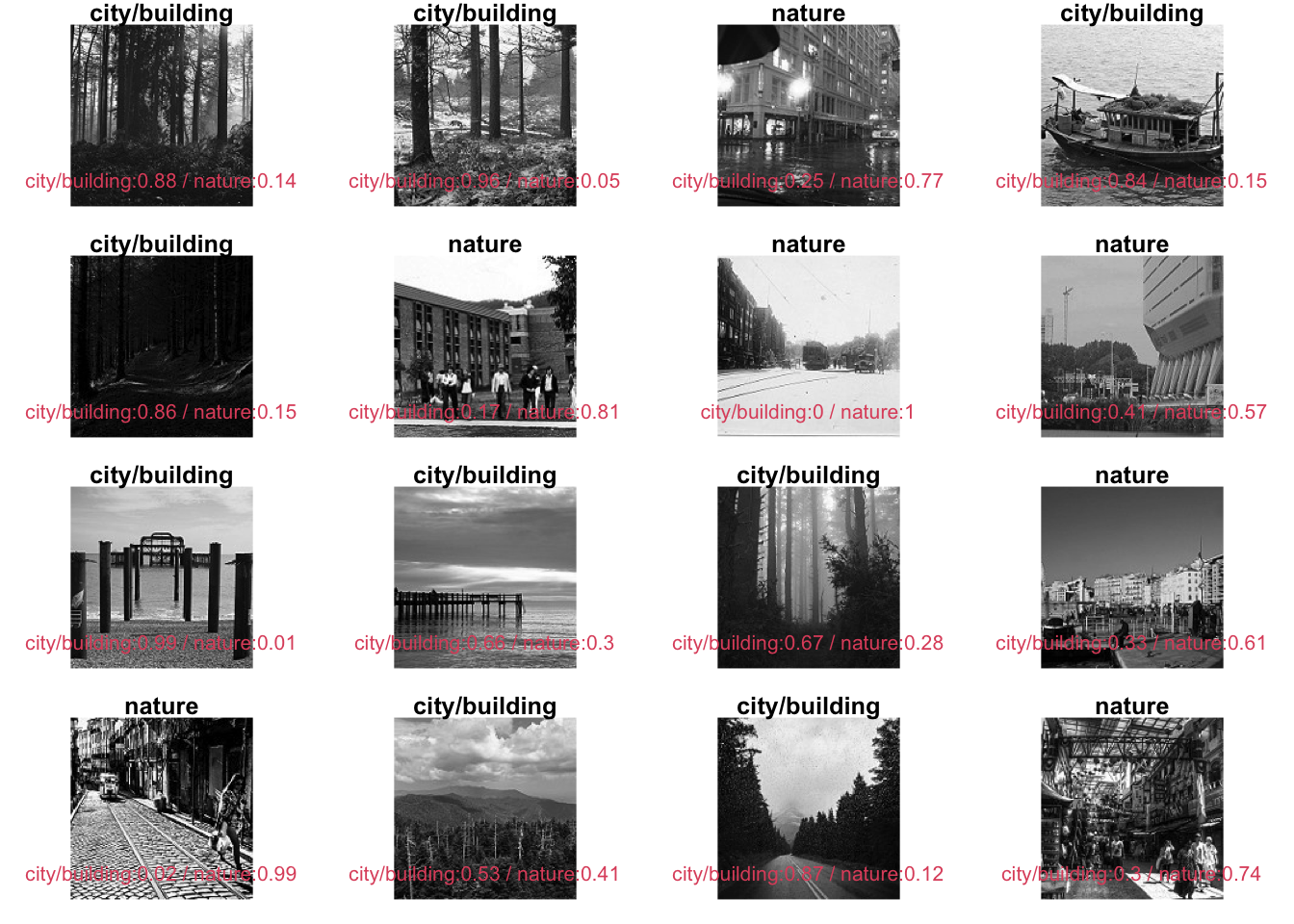
Looking at some of these examples it seems like often when the model makes a mistake it is in fact not very sure about the prediction. 43% / 57% split in label probabilities. Other cases raise questions about the correctness of labels. Most worrying however are instances where the model is really certain about the prediction, though to a human eye it is obviously a miss-classification.

Validation on Unseen Images

To conclude this short exercise we apply the model to a set of unlabeled images to see how well in works on images that were not use for either learning and testing during the training period.

val_image_files = list.files(paste0(path,"/data/seg_pred/seg_pred"), 
                             recursive = TRUE, 
                             full.names = TRUE)

val_data = map(val_image_files[1:400],
                ~image_load(.x, target_size = c(150,150), grayscale = TRUE) %>%
                  image_to_array() %>%
                  magrittr::divide_by(255)
)

X_val = 
  array(unlist(val_data), 
        dim = c(150, 150, 1, length(val_data))) %>% 
  aperm(c(4,1,2,3))

par(mfrow = c(2,2), mar = c(1,1,1,1))
as.cimg(X_val[1, , , ]) %>% imrotate(90) %>% plot(axes = FALSE)
as.cimg(X_val[2, , , ]) %>% imrotate(90) %>% plot(axes = FALSE)
as.cimg(X_val[3, , , ]) %>% imrotate(90) %>% plot(axes = FALSE)
as.cimg(X_val[4, , , ]) %>% imrotate(90) %>% plot(axes = FALSE)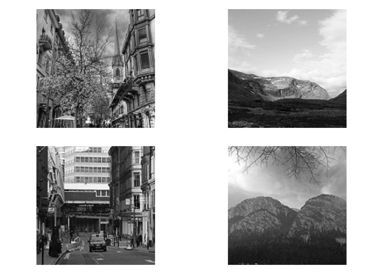

smodel = load_model_hdf5(paste0(path,"/tf_models/binary_gray_img_classification"), 
                         compile = TRUE)

vpred = vector(mode = "character", length = dim(X_val)[1])
for(i in 1:dim(X_val)[1]){
  vpred[i] = c("city/building","nature")[
    which.max(smodel %>% predict(X_val[i, , , ,drop = FALSE]))
    ]
}

set.seed(123)

par(mfrow = c(4,4), mar = c(1,1,1,1))
ri = sample(1:length(vpred), 16)
map(ri, ~ as.cimg(X_val[.x, , , ]) %>% 
      imrotate(90) %>% 
      plot(axes = FALSE, main = vpred[.x]))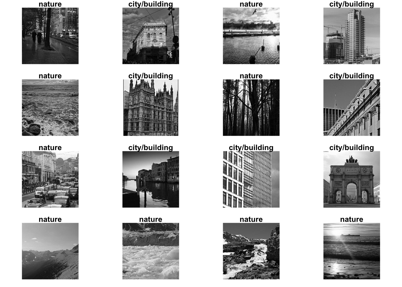

## [[1]]
## Image. Width: 150 pix Height: 150 pix Depth: 1 Colour channels: 1 
## 
## [[2]]
## Image. Width: 150 pix Height: 150 pix Depth: 1 Colour channels: 1 
## 
## [[3]]
## Image. Width: 150 pix Height: 150 pix Depth: 1 Colour channels: 1 
## 
## [[4]]
## Image. Width: 150 pix Height: 150 pix Depth: 1 Colour channels: 1 
## 
## [[5]]
## Image. Width: 150 pix Height: 150 pix Depth: 1 Colour channels: 1 
## 
## [[6]]
## Image. Width: 150 pix Height: 150 pix Depth: 1 Colour channels: 1 
## 
## [[7]]
## Image. Width: 150 pix Height: 150 pix Depth: 1 Colour channels: 1 
## 
## [[8]]
## Image. Width: 150 pix Height: 150 pix Depth: 1 Colour channels: 1 
## 
## [[9]]
## Image. Width: 150 pix Height: 150 pix Depth: 1 Colour channels: 1 
## 
## [[10]]
## Image. Width: 150 pix Height: 150 pix Depth: 1 Colour channels: 1 
## 
## [[11]]
## Image. Width: 150 pix Height: 150 pix Depth: 1 Colour channels: 1 
## 
## [[12]]
## Image. Width: 150 pix Height: 150 pix Depth: 1 Colour channels: 1 
## 
## [[13]]
## Image. Width: 150 pix Height: 150 pix Depth: 1 Colour channels: 1 
## 
## [[14]]
## Image. Width: 150 pix Height: 150 pix Depth: 1 Colour channels: 1 
## 
## [[15]]
## Image. Width: 150 pix Height: 150 pix Depth: 1 Colour channels: 1 
## 
## [[16]]
## Image. Width: 150 pix Height: 150 pix Depth: 1 Colour channels: 1

Next will try to fit a similar model but using colored images to see if that improves model accuracy.