Singular Value Decomposition
The SVD is one of the most useful matrix decomposition when it comes to Data Science. It’s used in practice for solving regression problems, various dimensionality reduction techniques including PCA, recommendation systems, image processing, and the list goes on.
My favorite thing about the SVD is that once you have the fundamentals of Linear Algebra down the SVD becomes pretty intuitive and easy to remember. I even coded it up myself with Rcpp - though admittedly my function is not as robust as what you will get with the out of the box functions in R or Python.
A Nib of Math
\[A = UΣV^T\]
This is it. The SVD gives us a way to decompose a rectangular - not necessarily square matrix - into three components. \(U\) and \(V^T\) are Orthogonal which is fantastic, and \(Σ\) is a Diagonal matrix of singular values in the descending order of magnitude. In geometric terms we decompose a multiplication by A into a rotation - scaling - rotation.
Here is a quick example in R:
First we simulate a 7 by 3 matrix of standard normal samples.
Then we simply use the svd function.
set.seed(007)
A = matrix(rnorm(21), ncol = 3)
A
## [,1] [,2] [,3]
## [1,] 2.2872472 -0.1169552 1.896067067
## [2,] -1.1967717 0.1526576 0.467680511
## [3,] -0.6942925 2.1899781 -0.893800723
## [4,] -0.4122930 0.3569862 -0.307328300
## [5,] -0.9706733 2.7167518 -0.004822422
## [6,] -0.9472799 2.2814519 0.988164149
## [7,] 0.7481393 0.3240205 0.839750360rsvd = svd(A)
rsvd## $d
## [1] 4.656225 3.134693 1.499431
##
## $u
## [,1] [,2] [,3]
## [1,] -0.32656110 0.81352961 0.105143318
## [2,] 0.14791225 -0.08172208 -0.710305948
## [3,] 0.49954916 -0.01632699 0.543434773
## [4,] 0.11901476 -0.09162081 0.031963386
## [5,] 0.60191049 0.21101396 0.116849337
## [6,] 0.49322511 0.37914465 -0.417596748
## [7,] -0.04689022 0.36681409 0.005149803
##
## $v
## [,1] [,2] [,3]
## [1,] -0.5168149 0.5480927 0.6576448
## [2,] 0.8467329 0.4405672 0.2982347
## [3,] -0.1262764 0.7109817 -0.6917798This function returns the UU and the VV matrices as well as a vector of singular values, which are the diagonal entries of ΣΣ
We can check that the product of matrices gives back the original matrix.
#A = UDV'
all.equal(rsvd$u %*% diag(rsvd$d) %*% t(rsvd$v), A)
## [1] TRUEAnd that the UU and the VV matrices are orthogonal
#Orthogonal
round(t(rsvd$u) %*% rsvd$u)
## [,1] [,2] [,3]
## [1,] 1 0 0
## [2,] 0 1 0
## [3,] 0 0 1round(rsvd$v %*% t(rsvd$v))## [,1] [,2] [,3]
## [1,] 1 0 0
## [2,] 0 1 0
## [3,] 0 0 1Application: Image Processing
A pretty cool and simple application of SVD is a deconstruction of images into layers of information.
If we look at a digital image as a two dimensional matrix and apply the SVD we will be able to reconstruct the image by taking the product of the three matrices.
However, if we want to reduce the data but loose as little information as possible we may take only a subset of singular values and their respective vectors from the UU and VV matrices.
Here is a concrete example using an image of an Aston Martin DB5 on display at the 007 exhibition at SPYSCAPE - the Spy Museum in NYC.
library(imager)## Loading required package: magrittr##
## Attaching package: 'imager'## The following object is masked from 'package:magrittr':
##
## add## The following objects are masked from 'package:stats':
##
## convolve, spectrum## The following object is masked from 'package:graphics':
##
## frame## The following object is masked from 'package:base':
##
## save.imageaston = load.image("../../../static/images/aston-db5.jpg")
aston_mat = aston[,,2]
aston_decomp = svd(aston_mat)
par(mfrow = c(4,4), mar = c(1,1,1,1))
plot(aston, axes = FALSE, main = "original image")
for(i in seq(2, 30, by = 2)){
n = i
reduced_img = as.cimg(aston_decomp$u[,1:n] %*% diag(aston_decomp$d[1:n]) %*% t(aston_decomp$v[,1:n]))
plot(reduced_img, axes = FALSE, main = paste(i))
}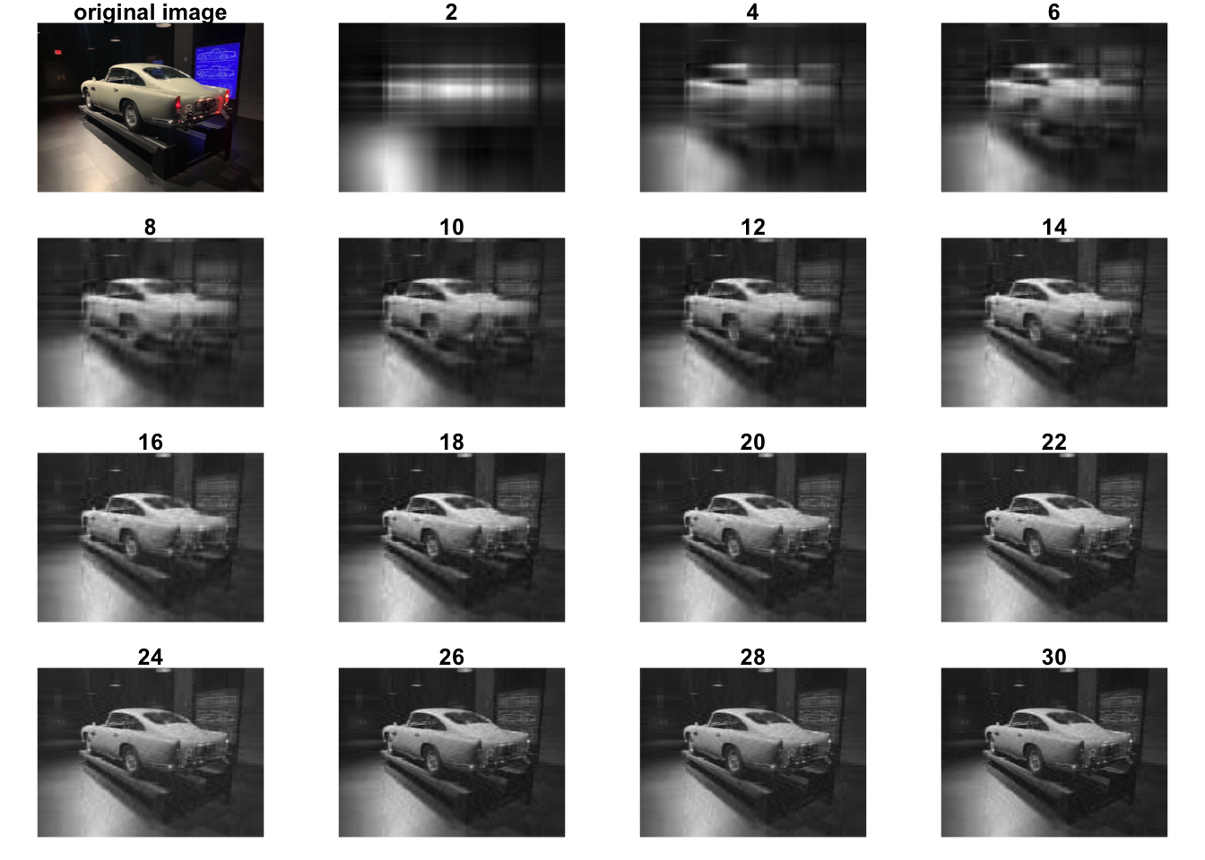
In the above code we load the image, apply the SVD to a grayscale version, and the reconstruct the image with an increasingly large subsets of the singular values.
Perhaps with only 4 dimensions we can’t yet recognize that this is an image of a car, but with just two more we can clearly see the vehicle.
If all we care to know is that the image contains a car, then 6-10 components are enough.
If for example we are bundling a classification model than this kind of data reduction may be a very useful pre-processing step.
A Bit More Math and Computation
So SVD seems pretty cool but how does it actually work? How is it computed?
The idea that helps me remember how SVD works is that SVD allows us to kind of invert a rectangular matrix - and it does so by applying the Eigen decomposition to two related square matrices. Given an \(A_{n,m}\) we can compute
\[ AA^T=M_{n,n} \] \[ AA^T=M{m,m} \]
Then if we decompose using, say the QR method, we will get the following
\[M_{n,n}=UΛ_nU^T, M_{m,m}=VΛ_mV^T\]
With this in mind it becomes relatively simple to compute the decomposition provided we know the eigenvlue decomposition. In practice we don’t only need to do one egenvalue decomposition as long as we are mindful of the dimensions of the input matrix. Here is an implementation in C++ and a check that it works.
List myc_svd(NumericMatrix A, double margin = 1e-20)
  int ncol = A.cols();
  int nrow = A.rows();
  if(ncol >= nrow){
    NumericMatrix X = myc_matmult(A, transpose(A));
    List E = myc_eigen(X);
    NumericVector d = E["values"];
    d = sqrt(d);
    NumericMatrix U = E["vectors"];
    NumericMatrix S(d.length(), d.length());
    for(int i = 0; i < d.length(); i++){
      for(int j = 0; j < d.length(); j++)
        if(i == j){
          S(i,j) = 1.0/d(i);
        }
    }
    NumericMatrix O = myc_matmult(transpose(U),A);
    NumericMatrix V = myc_matmult(S, O);
    V = transpose(V);
    List L = List::create(Named("d") = d,
                          Named("U") = U,
                          Named("V") = V,
                          Named("S") = S);
    return L;
  }else{
    NumericMatrix X = myc_matmult(transpose(A), A);
    List E = myc_eigen(X);
    NumericVector d = E["values"];
    d = sqrt(d);
    NumericMatrix V = E["vectors"];
    NumericMatrix S(d.length(), d.length());
    for(int i = 0; i < d.length(); i++){
      for(int j = 0; j < d.length(); j++)
        if(i == j){
          S(i,j) = 1.0/d(i);
        }
    }
    NumericMatrix O = myc_matmult(A,V);
    NumericMatrix U = myc_matmult(O,S);
    List L = List::create(Named("d") = d,
                          Named("U") = U,
                          Named("V") = V,
                          Named("S") = S);
    return L;
  }
}
library(myc)
mysvd = myc_svd(A)
all.equal(mysvd$U %*% diag(mysvd$d) %*% t(mysvd$V), A)## [1] TRUEmysvd## $d
## [1] 4.656225 3.134693 1.499431
##
## $U
## [,1] [,2] [,3]
## [1,] 0.32656148 0.81352927 -0.105143318
## [2,] -0.14791229 -0.08172192 0.710305948
## [3,] -0.49954917 -0.01632648 -0.543434773
## [4,] -0.11901480 -0.09162069 -0.031963386
## [5,] -0.60191039 0.21101458 -0.116849337
## [6,] -0.49322493 0.37914516 0.417596748
## [7,] 0.04689039 0.36681404 -0.005149803
##
## $V
## [,1] [,2] [,3]
## [1,] 0.5168153 0.5480924 -0.6576448
## [2,] -0.8467326 0.4405678 -0.2982347
## [3,] 0.1262769 0.7109816 0.6917798
##
## $S
## [,1] [,2] [,3]
## [1,] 0.2147663 0.0000000 0.0000000
## [2,] 0.0000000 0.3190105 0.0000000
## [3,] 0.0000000 0.0000000 0.6669196