What is Attribution Modeling
Attribution modeling is a task that comes up in Digital Marketing. Broadly speaking the objective of Attribution modeling is to improve the assessment of various Advertising Channels in driving Marketing Objectives. Before jumping to the data analysis let’s first set the context for the problem that Markov Chain Attribution modeling addresses.
With this post I am aiming to cover the following:
What is Attribution Modeling?
What is Multi-Touch Attribution?
Intro to Markov Chains
Using R for:
Simulating Consumer Journeys from a Markov Chain
Estimating a Markov Chain from Consumer Journeys
Using Markov Chains for Data-Driven Attribution
Many Advertising Channels
When marketers spend money on advertising they strategically allocate budget towards different campaigns which in turn use a multitude of advertising channels. Some common adverting channels include cable and streaming TV, Programmatic, Social, Paid Search, Print. How these are defined, and which media partners and platforms are used to spend the planned budget varies, but the fact that advertisers communicate through a multitude of channels remains.
Goals and KPI’s
Let’s keep in mind that marketers don’t advertise for the sake of advertising. They have particular goals and objectives around which a marketing communications strategy is built. One of the roles of Analytics is to help build a measurement plan that will define a set of Key Performance Indicators (KPI’s) that will serve as a measure of success for the marketing efforts. Depending on the goals, and technical ability these KPIs are chosen and tools for measuring them are put in place. For example, we may want to:
Generate visits to a website or a webpage
Generate leads through form submissions
Have users perform certain actions on our website
Raise awareness for our brand
or simply Drive sales
Whatever the KPI is, a unit of a completed KPI is referred to as a Conversion.
ROI and Attribution
While we are running a campaign and spending our budget there is a key question that we need to answer:
Obviously, if our goal was to drive sales but all else being equal our sales did not increase, then none of the channels worked well. But if we do succeed in driving incremental sales, which channel is working best? In other words, how do we Attribute the incremental sales to different channels and compute our Return on Investment (ROI, sometimes referred to as return on advertising (ROAS))? Should we tactically alter our plan because one of the channels is not performing as expected? Answering these questions is one-way Analytics ads value to Advertising.
Last-Touch in the Consumer Path
With Digital advertising our ability to measure when and how consumers interact with ads has become easier. This tractability allows us to collect data and analyze parts of the Consumer Path to a Conversion. A consumer journey exists whether or not it’s tracked, and no one can ever really track the whole journey. What we can track are some of the Media Touchpoints. Often the easiest way to Attribute Conversions is to simply look at the Last-Touch in the Consumer Path. That’s because by default this is the only touchpoint we do see. Giving the Last-Touch full credit for driving a Conversion will result in an unfair assessment of our media effectiveness and will not account for the Synergy that a mix of channels aims to create.
Thankfully if an adequate effort to track our media is made we can generate Path Data and hope to attribute in a more sophisticated way, that is using Multi-Touch Attribution (MTA). This allows us to better judge the effectiveness of channels used, and make better investment decisions.
Multi-Touch Attribution
There are two main categories of MTA methods; Rule-Based and Data-Driven. Of course, both of these use data but what distinguishes them is how they assign importance to touch-points along the consumer path. Rule-Based methods heuristically assign weights to touch-points based on their position.
Data-Driven methods take a different approach. Instead of assigning arbitrary rules based on the position they establish probabilistic relationships between touchpoints and their role in driving Conversions.
Markov Chain Attribution
Markov Chain Attribution is one of the more popular data-driven methods, and as the name suggests it takes advantage of Markov Chains. Unless you studied Operations Research or Math at university you might not know what these chains are so let’s do a high-level intro.
Markov Chains
The key concept to remember about Markov Chains is the Transition Matrix. Markov Chains themselves are a conceptual tool for describing a (stochastic) system. All this means is that when there is randomness or a probabilistic component to a process, Markov Chains might be a good tool to first describe, and then analyze this process. The process we are concerned with here is Customer Journeys towards Conversions.
The Fundamentals
We can visualize a Markov Chain as a directed network. Each node is a State that a consumer can be in while following a path. Each arrow is a Transition, and with it, there is an associated probability. So there is a predetermined set of touch-points you may have, but which will happen next is uncertain.
library(visNetwork)
library(tidyverse)
library(gt)
nodes <-
  data.frame(id = 1:6,
             label = c("Non-Conversion", "Display", "TV",
                       "Search", "Conversion","Start"),
             color = c("darkred", "grey", "grey",
                       "grey", "lightblue", "green"))
edges = expand.grid(from = 1:6, to = 1:6)
edges = edges %>% filter(from != to, to != 5, to != 1, from != 6)

visNetwork(nodes, edges, width = "100%") %>%
  visEdges(arrows = "from") %>%
  visIgraphLayout(layout = "layout_with_kk")
The conversion and non-conversion nodes have arrows pointing to them from all channels, but no arrows emanating from them. These are called Absorbing States and for us, they indicate an end of a journey. When we collect all of the probabilities of transitioning from one state to the next, we organize them in a square Transition Matrix.
M = t(matrix(c(1,    0,   0,   0,  0,
               200,   0, 300, 350, 10,
               160, 300,   0, 350,  8,
               150, 200, 200,   0,  20,
               0,    0,   0,   0,  1), nrow = 5))

M = M/rowSums(M)

colnames(M) = c("Non-Conversion", "Display","TV","Search","Conversion")
row.names(M) = c("Non-Conversion", "Display","TV","Search","Conversion")

as.data.frame(round(M,3), row.names = row.names(M)) %>%
  rownames_to_column() %>% gt::gt() %>%
  gt::tab_header(title = "Theoretical Transition Matrix")  %>%
  tab_style(style = list(cell_fill(color = "#F1CBC3")),
            locations = cells_body(columns = c(2,6), rows = 2:4)) %>%
  tab_style(style = list(cell_fill(color = "#F6A392")),
            locations = cells_body(columns = 3, rows = 3:4)) %>%
  tab_style(style = list(cell_fill(color = "#F6A392")),
            locations = cells_body(columns = 4, rows = c(2,4))) %>%
  tab_style(style = list(cell_fill(color = "#F6A392")),
locations = cells_body(columns = 5, rows = 2:3))| Theoretical Transition Matrix | |||||
|---|---|---|---|---|---|
| Non-Conversion | Display | TV | Search | Conversion | |
| Non-Conversion | 1.000 | 0.000 | 0.000 | 0.000 | 0.000 |
| Display | 0.233 | 0.000 | 0.349 | 0.407 | 0.012 |
| TV | 0.196 | 0.367 | 0.000 | 0.428 | 0.010 |
| Search | 0.263 | 0.351 | 0.351 | 0.000 | 0.035 |
| Conversion | 0.000 | 0.000 | 0.000 | 0.000 | 1.000 |
Above is an example Transition Matrix which I just put together for illustration. To make it realistic I set the conversions probabilities to relatively low values. Later we will use this matrix for Simulation!
An important property to keep in mind is that rows sum up to one since we are dealing with probabilities. The rows represent the current state in the journey, and columns represent the next state.
rowSums(M)## Non-Conversion Display TV Search Conversion
## 1 1 1 1 1There is one more important thing to know about Markov Chains, and that is the Markov Property or the memorylessness. This will be TMI for some, but this is really the reason why it is possible to summarize the whole process in one simple Transition Matrix. The property is a simplifying assumption stating that the probability of where you transition to next depends only on where you are now, but not on your whole journey history. To be clear, this doesn’t mean that the journey history doesn’t matter. It absolutely does impact attribution results. What it doesn’t impact is the probability. This makes analysis significantly simpler from a mathematical point of view.
From Chains to Paths (Simulation)
In practice, given a data-set of consumer paths (constructing this data-set is a big task so ‘given’ is a strong word), we may estimate a Transition Matrix. The reverse is also true. Given a Transition Matrix we can simulate a set of consumer paths. In fact, simulation plays an important role in deriving the actual levels of importance for each channel, so it is worth seeing the mechanics of this process.
Below we define a function that will work well with the above sample matrix \(M\). Given this matrix and a number of Markov Chain steps we want to make num_sim we do the following:
Randomly select a starting point by sampling from the set of media touchpoints
- In practice we would actually estimate the starting point probabilities.
For each step:
Pick a row of probabilities from \(M\) corresponding to the current state/touchpoint.
- Take one sample from a
Multinomialdistribution with probabilities set to the row.
- Take one sample from a
Set the sample as the new current state and repeat.
If we hit a
ConversionorNon-Conversionwe end the path.
simulate_path = function(M, num_sim){
  num_sim = num_sim
  path = vector(mode = "integer", length = num_sim)
  path[1] = sample(2:(nrow(M)-1), 1)
  for(i in 1:(num_sim-1)){
    p = M[path[i],]
    sn = which(rmultinom(1, 1, p) == 1)
    path[i+1] = sn
    if(sn == 1 | sn == 5){
      break
    }
  }
  return(path[path > 0])
}
Simulating One Path
Let’s test out this function. The first example is a non-converter.
set.seed(124)
num_sim = 100
path = simulate_path(M, num_sim)
plot(seq_along(path), path ,
     type = "l", axes=FALSE, ylim = c(1,5),
     main = "Non-Converter",
     ylab = "Channel Touchpoint",
     xlab = "Touchpoint Number")
points(seq_along(path), path)
axis(side = 2, at = 1:5)
axis(side = 1, at = seq_along(path))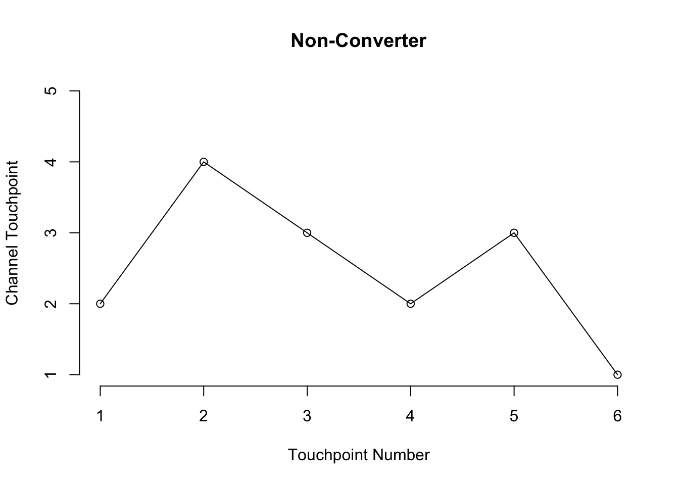
We see that we start out with Display, move to Search, then TV, carry on the journey until step 6 where we drop out without converting.
This is another example but this time we have a converter.
set.seed(007)
num_sim = 100
path = simulate_path(M, num_sim)
plot(seq_along(path), path ,
     type = "l", axes=FALSE, ylim = c(1,5),
     main = "Converter",
     ylab = "Channel Touchpoint",
     xlab = "Touchpoint Number")
points(seq_along(path), path)
axis(side = 2, at = 1:5)
axis(side = 1, at = seq_along(path))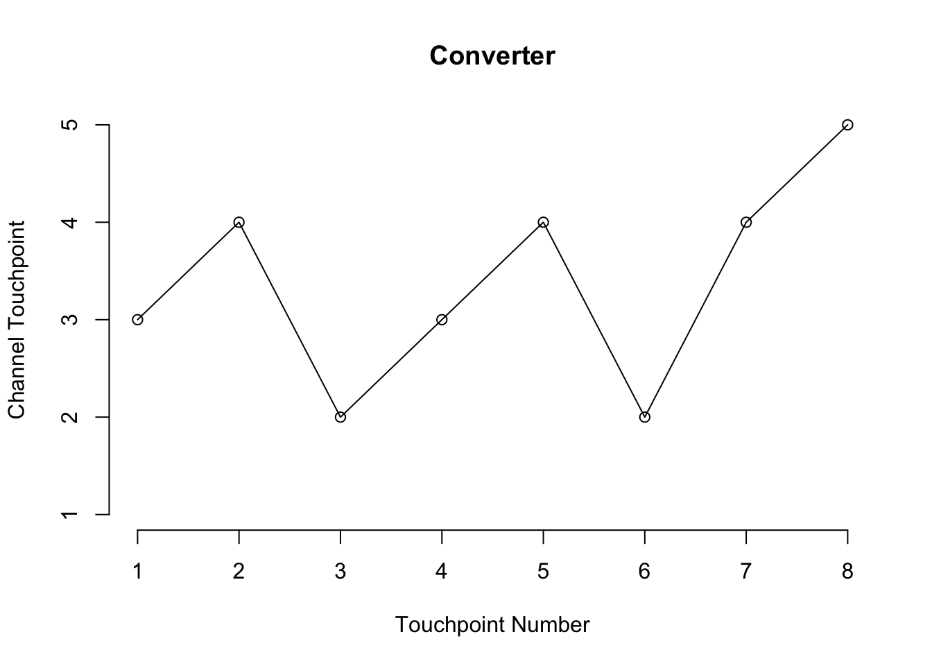
This time we started out with TV and converted on step 8 with Search being our last touchpoint.
Simulating a Full Data-set of Journeys
We can now simulate a whole set of paths simply by repeating the function call simulate_path. With a few more data wrangling operations we have a pathdf. Here I will generate 10,000 paths.
num_sim = 100
num_paths = 10000

paths = purrr::map(1:num_paths, ~simulate_path(M, num_sim))

conversion =
  purrr::map(paths, ~ data.frame(conversion =
                                   ifelse(.x[length(.x)] == 5,
                                          "converter",
                                          "non-converter")
                                 )
             ) %>% bind_rows(.id = "path_num")

pathdf =
  map(paths, ~data.frame(touchpoint = 1:length(.x), channel = .x)) %>%
  bind_rows(.id = "path_num") %>%
  left_join(conversion) %>%
  left_join(
    data.frame(channel_name = colnames(M), channel = 1:5)
  )

head(pathdf,10) %>% gt::gt() %>%
gt::tab_header(title = "Simmulated Paths")| Simmulated Paths | ||||
|---|---|---|---|---|
| path_num | touchpoint | channel | conversion | channel_name |
| 1 | 1 | 4 | non-converter | Search |
| 1 | 2 | 2 | non-converter | Display |
| 1 | 3 | 1 | non-converter | Non-Conversion |
| 2 | 1 | 4 | non-converter | Search |
| 2 | 2 | 2 | non-converter | Display |
| 2 | 3 | 3 | non-converter | TV |
| 2 | 4 | 2 | non-converter | Display |
| 2 | 5 | 4 | non-converter | Search |
| 2 | 6 | 2 | non-converter | Display |
| 2 | 7 | 3 | non-converter | TV |
Let’s now plot all of these paths on top of one another to see how this Markov Chain behaves.
plotly::ggplotly(
pathdf %>%
  ggplot(aes(touchpoint, channel, color = conversion, group = path_num)) +
  geom_line() +
  labs(x = "Touchpoint Number", y = "Channel Touhcpoint") +
  theme_minimal()
)
From the plot we see that more often lines drop down, which indicates a non-converter. This is as expected. We can see that the simulated conversion rate was just over 8%.
table(conversion$conversion)/nrow(conversion)##
## converter non-converter
## 0.0808 0.9192From Paths to Chains
Now that we have simulated a set of consumer paths from our Markov Chain \(M\) we can try to use them to estimate the original \(M\) with \(\hat{M}\) and see how well the estimation method works. Here I will introduce the brilliant ChannelAttribution package authored by Davide Altomare. It is open source and hosted on GitLab here. This package contain a function called transition_matrix which takes in a data-set of paths and estimates the Transition Matrix.
Data Prep
The first order of business is to structure the data in the required format. First we need to parse out the final touchpoint in each path since they represent a conversion/non-conversion event. Then we summarize the data grouping by path and count the number converters and non-converters for each unique path observed.
named_paths =
  pathdf %>% group_by(path_num) %>%
  group_split() %>%
  map(~pull(.x,channel_name))

path_trim = map(named_paths, ~.x[.x != "Non-Conversion" & .x != "Conversion"])

journeydf =
  as_tibble(
    cbind(
      as.data.frame(
        do.call(rbind,
                map(path_trim, ~str_c(.x, collapse = " > "))
                )
        ),conversion$conversion)
    )

names(journeydf) = c("path","conversion")

journeydf =
  journeydf %>%
  group_by(path) %>%
  summarise(
    converters = sum(if_else(conversion == "converter", 1, 0)),
    non_converters = sum(if_else(conversion == "non-converter", 1, 0))
    ) %>%
  arrange(-converters, -non_converters)

head(journeydf, 15) %>% gt::gt() %>%
gt::tab_header(title = "Simmulated Journey Data (Top 15 Converters)")| Simmulated Journey Data (Top 15 Converters) | ||
|---|---|---|
| path | converters | non_converters |
| Search | 78 | 902 |
| Display | 60 | 804 |
| TV | 53 | 588 |
| Search > Display | 29 | 267 |
| TV > Search | 27 | 409 |
| Display > Search | 26 | 329 |
| Search > TV | 20 | 227 |
| Display > TV | 20 | 224 |
| TV > Display | 18 | 269 |
| TV > Search > Display | 14 | 104 |
| Display > TV > Search | 13 | 152 |
| Search > Display > Search | 13 | 127 |
| Display > Search > Display > Search | 10 | 50 |
| TV > Display > Search | 8 | 128 |
| TV > Search > TV | 8 | 95 |
Here are some quick summary stats about the generated path data.
data.frame(
  metric = c("Converters",
             "Non Converters",
             "Number of Paths",
             "Conversion Rate %",
             "Unique Journeys"),
  value = c(sum(journeydf$converters),
            sum(journeydf$non_converters),
            sum(journeydf$non_converters) + sum(journeydf$converters),
            100*sum(journeydf$converters) / num_paths,
            nrow(journeydf))) %>%
  gt::gt() %>%
gt::tab_header(title = "Summary")| Summary | |
|---|---|
| metric | value |
| Converters | 808.00 |
| Non Converters | 9192.00 |
| Number of Paths | 10000.00 |
| Conversion Rate % | 8.08 |
| Unique Journeys | 1501.00 |
There are many other ways to explore this kind of data. One quick and intersection one is the distribution of path lengths.
path_lengths = map_int(path_trim, ~length(.x))
summary(path_lengths)
## Min. 1st Qu. Median Mean 3rd Qu. Max.
## 1.000 2.000 3.000 4.002 5.000 31.000hist(path_lengths, main = "Path Length Distribution")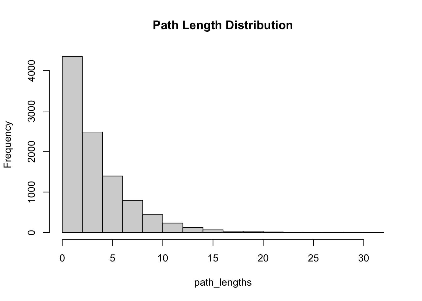
Transition Matrix Estimation
Finally, now that we have our simulated data-set with a known transition matrix \(M\) , we can now see how we can go from data back to a transition matrix, via estimation and compute \(\hat{M}\). Here we apply the ChannelAttribution::transition_matrix() function to out data. The function returns a lookup table for the channel ids and a table to transition probabilities.
library(ChannelAttribution)

tM = transition_matrix(journeydf,
                       var_path = "path",
                       var_conv = "converters",
                       var_null = "non_converters")

tM$transition_matrix %>% gt::gt() %>%
gt::tab_header(title = "Transition Probabilities")| Transition Probabilities | ||
|---|---|---|
| channel_from | channel_to | transition_probability |
| (start) | 1 | 0.33580000 |
| (start) | 2 | 0.33780000 |
| (start) | 3 | 0.32640000 |
| 1 | (conversion) | 0.02380785 |
| 1 | (null) | 0.27083187 |
| 1 | 2 | 0.35113052 |
| 1 | 3 | 0.35422977 |
| 2 | (conversion) | 0.02017868 |
| 2 | (null) | 0.22704868 |
| 2 | 1 | 0.40280345 |
| 2 | 3 | 0.34996919 |
| 3 | (conversion) | 0.01620316 |
| 3 | (null) | 0.18688167 |
| 3 | 1 | 0.43694010 |
| 3 | 2 | 0.35997507 |
We can format and the table and output in a way where it is easy for us to compare the estimated and the true transition matrices
| Estimated Transition Matrix | |||||
|---|---|---|---|---|---|
| (null) | Display | TV | Search | (conversion) | |
| Display | 0.227 | 0.000 | 0.350 | 0.403 | 0.020 |
| TV | 0.187 | 0.360 | 0.000 | 0.437 | 0.016 |
| Search | 0.271 | 0.351 | 0.354 | 0.000 | 0.024 |
| Original Transition Matrix | |||||
|---|---|---|---|---|---|
| Non-Conversion | Display | TV | Search | Conversion | |
| Display | 0.233 | 0.000 | 0.349 | 0.407 | 0.012 |
| TV | 0.196 | 0.367 | 0.000 | 0.428 | 0.010 |
| Search | 0.263 | 0.351 | 0.351 | 0.000 | 0.035 |
We can see that the estimation worked pretty well especially for the larger probabilities. Because conversion event are much rarer there is more variability / less precision for their estimates.
Attribution
So far we introduced a theoretical Markov Chain in the form of a transition matrix \(M\) , used it to simulate a data-set of Consumer Journeys, and returned back to a Transition Matrix by estimating \(\hat{M}\). Now it’s time to convert, and move on to the actually attribution model!
Removal Effects
Markov Chains seem to be a good idea as a model for Consumer Journeys. But how do we use them to actually attribute conversions is not immediately clear.
The main idea here is to compute Removal Effects. Removal Effects measure how many fewer conversions would be observed if a channel was omitted/removed from the paths. If we compute this for each channel in the Markov Chain then the Relative Removal Effects will be the factor by which we scale the total conversion volume.
Running Attribution
As we just learned running a Markov attribution model involves estimating a Transition Matrix and then computing the Removal Effects. To do this we simply use the markov_model function, which takes the data in the prepared format. By specifying out_more = TRUE in addition to the attribution results we also get back the transition matrix and removal effects.
mm_res =
  markov_model(journeydf,
             var_path = "path",
             var_conv = "converters",
             var_null = "non_converters",
             out_more = TRUE)
##
## Number of simulations: 100000 - Convergence reached: 2.32% < 5.00%
##
## Percentage of simulated paths that successfully end before maximum number of steps (32) is reached: 99.98%Attribution Results
First, let’s take a look at the results. The total number of conversions was 808. The below table shows how these were attributed by our Data-Driven model.
mm_res$result %>% gt::gt() %>%
gt::tab_header(title = "Markov Chain Attribution Results")| Markov Chain Attribution Results | |
|---|---|
| channel_name | total_conversions |
| Search | 284.9682 |
| Display | 263.2859 |
| TV | 259.7459 |
We see that the number of conversions attributed to each channel is similar however Search was attributed the most conversions. This is not surprising since transition probabilities were steered towards Search but only slightly. In addition, each channel was equally likely to be picked as a first touchpoint in our simulation which doesn’t happen in reality.
To show how these results are calculated from the removal effects here is the explicit code:
total_coversions = sum(journeydf$converters)
removal_effects =  mm_res$removal_effects$removal_effects
relative_removal_effects = removal_effects/sum(removal_effects)
attributed_conversions = total_coversions * relative_removal_effects

attributed_conversions
## [1] 284.9682 263.2859 259.7459The removal effects themselves can be easily accessed and interpreted
removal_effects## [1] 0.7806061 0.7212121 0.7115152From these numbers, we see that about 78% fewer conversions would be observed if Search was removed. This is quite dramatic but not surprising for such a small and interconnected Markov Chain.
Quick Comparison to Rule-Based Models
With the ChannelAttribution package it is easy to also get results of some Rule-Based models and compare them to the Data-Driven results.
mta_res =
  heuristic_models(journeydf,
                 var_path = "path",
                 var_conv = "converters") %>%
  left_join(mm_res$result)
## Joining, by = "channel_name"mta_res %>% gt::gt() %>%
gt::tab_header(title = "MTA Model Result Comparison")| MTA Model Result Comparison | ||||
|---|---|---|---|---|
| channel_name | first_touch | last_touch | linear_touch | total_conversions |
| Search | 282 | 338 | 299.0591 | 284.9682 |
| Display | 269 | 262 | 262.9943 | 263.2859 |
| TV | 257 | 208 | 245.9466 | 259.7459 |
We can clearly see the difference between Last-Touch and the Markov Chain model results as the importance of Display and especially TV are well underestimated. Last-Touch attributed 50 fewer conversions to TV than the Markov Chain model. This example makes it clear how Markov Chain attribution can correct for the inherent bias of the Last-Touch attribution. Linear Touch results are similar here, again because the transition probabilities are quite between the channels are not too far apart.
mta_res %>%
  pivot_longer(-channel_name, names_to = "MTA_Model", values_to = "Conversions") %>%
  ggplot(aes(MTA_Model, Conversions, fill = channel_name)) +
  geom_col(position = "dodge") +
  labs(title = "MTA Model Result Comparison") +
  theme_minimal()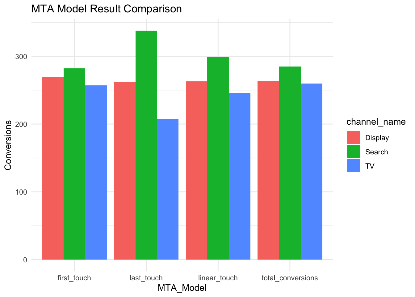
Key Considerations
Hopefully, you find the topic of MTA and Markov Chain Attribution as interesting as I do. Though this introduction is quite lengthy there are still many aspects of this type of analysis to consider. Here are a few crucial things that need to be considered next:
Data is the key ingredient of any data analysis so the quality of analysis hinges on the quality of data.
Quality of data depends on a few factors:
Measurability — how well can a Channel be measured? Digital ads are easily measured while OOH (street banners) are hard to track.
Measurement — just because something is easy to measure doesn’t mean it is well measured. If proper tools are not implemented, maintained, and managed data will not be properly collected.
Data Management — even if data is properly collected it still needs to be managed which means naming conventions and data classification has to be in place.
Cross-Device / Cross-Platform (Walled Gardens) — in order to stitch together the
Customer Journeydata we need to be able to identify users across different platforms and devices through which they are reached. This is perhaps the biggest limitation of MTA today.
3. The Data Engineering aspect is important if MTA results need to be delivered frequently and efficiently. The more flexibility the more complexity there will be.
4. We might also want to consider if there are better ways to estimate the transitions matrix for example with Bayesian methods.